class: center, middle, inverse, title-slide # STA 506 2.0 Linear Regression Analysis ## Week 5: Multiple Linear Regression ### Dr Thiyanga S. Talagala --- ## Multiple Linear Regression - A regression model that involves **two or more independent variables** and **one dependent variable**. .content-box-blue[Simple Linear Regression `$$Y = \beta_0 + \beta_1X_1 + \epsilon$$` In terms of the observed values, `$$y_i = \beta_0 + \beta_1x_i + \epsilon_i \text{ ; } i=1, 2, ...n$$` ] .content-box-yellow[Multiple Linear Regression $$Y = \beta_0 + \beta_1X_1 + \beta_2X_2+...+\beta_pX_p + \epsilon $$ In terms of the observed values, `$$y_i = \beta_0 + \beta_1x_{i1} + \beta_2x_{i2}+...+\beta_px_{ip} + \epsilon_i \text{ ; } i=1, 2, ...n$$` ] --- ## Multiple Linear Regression `$$Y = \beta_0 + \beta_1X_1 + \beta_2X_2+...+\beta_pX_p + \epsilon$$` In terms of the observed values, `$$y_i = \beta_0 + \beta_1x_{i1} + \beta_2x_{i2}+...+\beta_px_{ip} + \epsilon_i \text{ ; } i=1, 2, ...n$$` ### Notation for the data in multiple regression analysis | Observation No. | Response | Predictor 1 | Predictor 2 |...|Predictor p |:-:|:-:|:-:|:-:|:-:|:-:| | | `\(Y\)` | `\(X_1\)` | `\(X_2\)` | ... | `\(X_p\)` | | 1 | `\(y_1\)` | `\(x_{11}\)` | `\(x_{12}\)` | ... | `\(x_{1p}\)` | | 2 | `\(y_2\)` | `\(x_{21}\)` | `\(x_{22}\)` | ... | `\(x_{2p}\)` | | 3 | `\(y_3\)` | `\(x_{31}\)` | `\(x_{32}\)` | ... | `\(x_{3p}\)` | | . | . | . | . | . .. | . | | n | `\(y_n\)` | `\(x_{n1}\)` | `\(x_{n2}\)` | ... | `\(x_{np}\)` | --- #### Multiple linear regression model with `\(p\)` predictors `$$y_i = \beta_0 + \beta_1x_{i1} + \beta_2x_{i2}+...+\beta_px_{ip} + \epsilon_i$$` > `\(y_i\)` represents the `\(i^{th}\)` value of the response variable `\(Y\)`. > `\(x_{i1}, x_{i2}, ...x_{ip}\)` represent values of the predictor variables for the `\(i^{th}\)` observation. > `\(\beta_0, \beta_1, ...\beta_p\)` are called the **partial regression coefficients**. #### Model assumptions 1. The relationship between the response `\(Y\)` and the predictors is linear, at least approximately. 2. The error term `\(\epsilon\)` has zero mean. 3. The error term `\(\epsilon\)` has constant variance `\(\sigma^2\)`. 4. The errors are uncorrelated. 5. The errors are normally distributed. Taken together, assumptions 4 and 5 imply that the errors are independent. Assumption 5 is required for hypothesis testing and interval estimation. --- ## Example: Crop yields prediction based on temperature and amount of fertilizer added. A multiple regression model that might describe this relationship is `\(Y = \beta_0 + \beta_1X_1 + \beta_2 X_2 + \epsilon\)` where, `\(Y\)` denotes the yield `\(X_1\)` denotes the temperature `\(X_2\)` denotes the amount of fertilizer added `\(\beta_0\)` denotes population intercept `\(\beta_1\)` denotes partial regression coefficient of the variable temperature `\(\beta_2\)` denotes partial regression coefficient of the variable amount of fertilizer added `\(\epsilon\)` random error term. --- ### Visualization .pull-left[ #### Simple linear regression 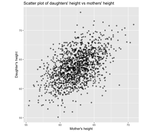<!-- --> ] .pull-right[ #### Multiple linear regression 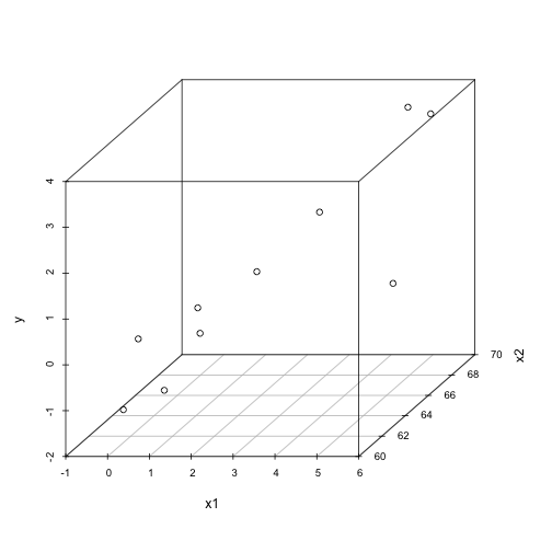<!-- --> ] --- ### Visualization .pull-left[ #### Simple linear regression <!-- --> ] .pull-right[ #### Multiple linear regression 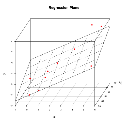<!-- --> ] Simple linear regression: **line of best fit** Multiple linear regression: **plane of best fit** > More than 2 independent variables: Hard to visualize. --- ### Visualization .pull-left[ #### Simple linear regression 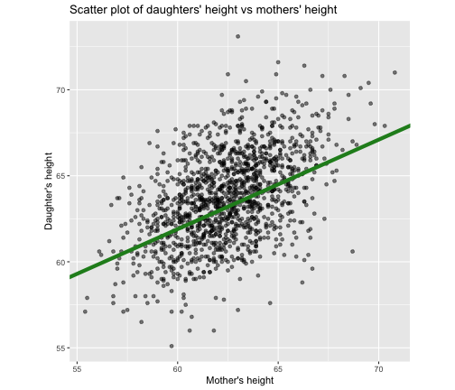<!-- --> ] .pull-right[ #### Multiple linear regression + Fitted values (blue) 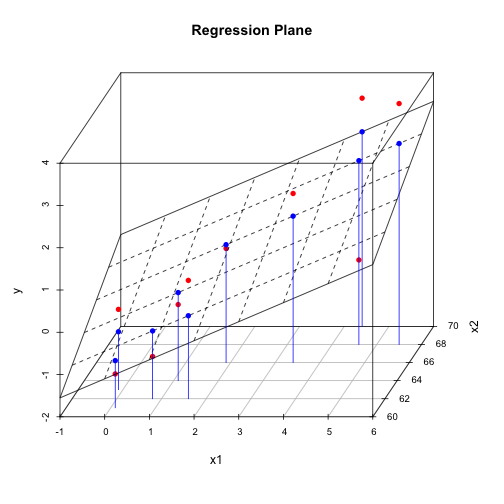<!-- --> ] Simple linear regression: **line of best fit** Multiple linear regression: **plane of best fit** More than 2 independent variables: Hard to visualize. --- ## Modelling steps 1. Exploratory Data Analysis 2. Fitting a models 3. Assess the model - How well it fits the data? - Is it useful? - Are any required conditions violated? 4. Employ the model - Interpreting the coefficients. - Predictions using the prediction equation. - Estimating the expected value of the dependent variable. --- # Example A public health researcher interested in social factors that influence heart disease. He surveyed 500 towns and gather data on the **percentage of people in each town who smoke**, **the percentage of people in each town who bike to work**, and **the percentage of people in each town who have heart disease**. Download the dataset from the course website: heart.data under week 8 [here](https://thiyanga.netlify.app/courses/regression2020/contentreg/). --- ## Read data into R ```r library(tidyverse) ``` ``` Warning: package 'tidyr' was built under R version 4.1.2 ``` ``` Warning: package 'readr' was built under R version 4.1.2 ``` ```r heart.data <- read_csv("heart.data.csv") heart.data ``` ``` # A tibble: 498 × 4 ...1 biking smoking heart.disease <dbl> <dbl> <dbl> <dbl> 1 1 30.8 10.9 11.8 2 2 65.1 2.22 2.85 3 3 1.96 17.6 17.2 4 4 44.8 2.80 6.82 5 5 69.4 16.0 4.06 6 6 54.4 29.3 9.55 7 7 49.1 9.06 7.62 8 8 4.78 12.8 15.9 9 9 65.7 12.0 3.07 10 10 35.3 23.3 12.1 # … with 488 more rows ``` --- ## Variable description <img src="dataheartdisease.png" width="50%" /> .red[X1] - Town ID .red[biking] - percentage of people in each town who bike to work .red[smoking] - percentage of people in each town who smoke .red[heart.disease] - percentage of people in each town who have heart disease --- ### Scatterplot matrix/ correlogram ```r library(GGally) # Make sure you install the package before running the code ggpairs(heart.data[,c("biking", "smoking", "heart.disease")]) ``` <!-- --> --- ### Scatterplot matrix/ correlogram .pull-left[ <!-- --> ] .pull-right[ Scatterplots of each pair of numeric variable are drawn on the left part of the figure. Pearson correlation is displayed on the right. Variable distribution is available on the diagonal. ] --- ### Scatterplot matrix/ correlogram .pull-left[ <!-- --> ] .pull-right[ ```r qplot(data=heart.data, x=biking) + geom_histogram(color="black", fill="#d95f02") ``` 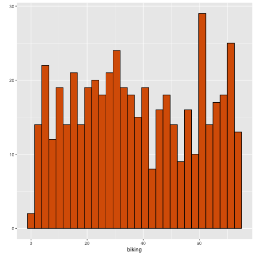<!-- --> ] --- ### Scatterplot matrix .pull-left[ <!-- --> ] .pull-right[ ```r qplot(data=heart.data, x=smoking) + geom_histogram(color="black", fill="forestgreen") ``` 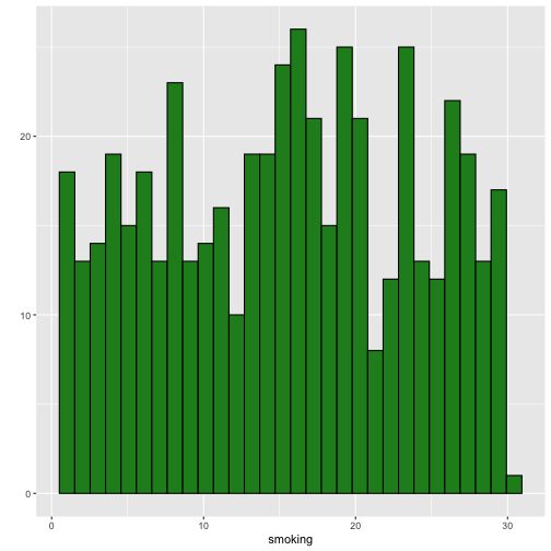<!-- --> ] --- ### Scatterplot matrix .pull-left[ <!-- --> ] .pull-right[ ```r qplot(data=heart.data, x=heart.disease) + geom_histogram(color="black", fill="yellow") ``` 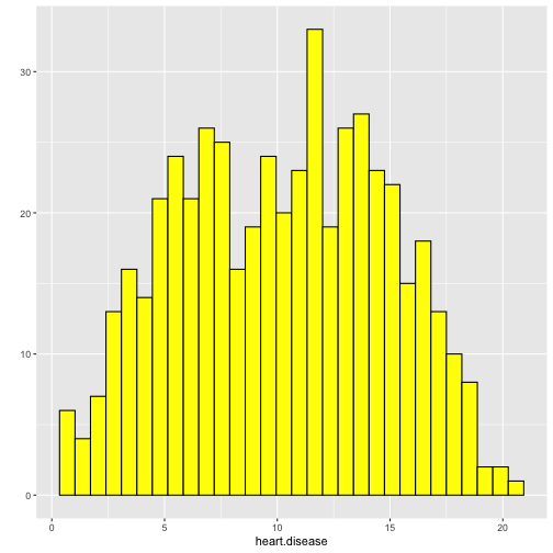<!-- --> ] --- ## Fit a regression model ```r regHeart <- lm(heart.disease ~ biking+ smoking, data=heart.data) regHeart ``` ``` Call: lm(formula = heart.disease ~ biking + smoking, data = heart.data) Coefficients: (Intercept) biking smoking 14.9847 -0.2001 0.1783 ``` -- .red[Fitted regression model] `\(\hat{Y} = 14.9847 - 0.2001X_1 + 0.1783X_2\)` where `\(\hat{Y}\)` - Fitted values `\(X_1\)` - percentage of people in each town who bike to work `\(X_2\)` - percentage of people in each town who smoke --- ## Model description ```r summary(regHeart) ``` ``` Call: lm(formula = heart.disease ~ biking + smoking, data = heart.data) Residuals: Min 1Q Median 3Q Max -2.1789 -0.4463 0.0362 0.4422 1.9331 Coefficients: Estimate Std. Error t value Pr(>|t|) (Intercept) 14.984658 0.080137 186.99 <2e-16 *** biking -0.200133 0.001366 -146.53 <2e-16 *** smoking 0.178334 0.003539 50.39 <2e-16 *** --- Signif. codes: 0 '***' 0.001 '**' 0.01 '*' 0.05 '.' 0.1 ' ' 1 Residual standard error: 0.654 on 495 degrees of freedom Multiple R-squared: 0.9796, Adjusted R-squared: 0.9795 F-statistic: 1.19e+04 on 2 and 495 DF, p-value: < 2.2e-16 ``` --- ### Regression Diagnostics (Model adequacy checking) .blue[ 1. The relationship between the response `\(Y\)` and the predictors is linear, at least approximately. 2. The error term `\(\epsilon\)` has zero mean. 3. The error term `\(\epsilon\)` has constant variance `\(\sigma^2\)`. 4. The errors are uncorrelated. 5. The errors are normally distributed. ] .red[ Is multicollinearity a problem?] --- ## Compute residuals and fitted values ```r library(broom) regHeart_values <- augment(regHeart) regHeart_values ``` ``` # A tibble: 498 × 9 heart.disease biking smoking .fitted .resid .hat .sigma .cooksd <dbl> <dbl> <dbl> <dbl> <dbl> <dbl> <dbl> <dbl> 1 11.8 30.8 10.9 10.8 1.01 0.00281 0.653 0.00223 2 2.85 65.1 2.22 2.35 0.508 0.0105 0.654 0.00216 3 17.2 1.96 17.6 17.7 -0.551 0.00777 0.654 0.00187 4 6.82 44.8 2.80 6.52 0.298 0.00693 0.655 0.000487 5 4.06 69.4 16.0 3.94 0.124 0.00638 0.655 0.0000770 6 9.55 54.4 29.3 9.33 0.222 0.00879 0.655 0.000344 7 7.62 49.1 9.06 6.78 0.842 0.00378 0.654 0.00210 8 15.9 4.78 12.8 16.3 -0.461 0.00693 0.654 0.00117 9 3.07 65.7 12.0 3.97 -0.901 0.00579 0.653 0.00371 10 12.1 35.3 23.3 12.1 0.0188 0.00384 0.655 0.00000107 # … with 488 more rows, and 1 more variable: .std.resid <dbl> ``` --- ## Residuals versus fitted values ```r qplot(data=regHeart_values, y=.resid, x=.fitted) ``` <!-- --> --- ### Regression Diagnostics (Model adequacy checking) .blue[ 1. The relationship between the response `\(Y\)` and the predictors is linear, at least approximately. ✅ 2. The error term `\(\epsilon\)` has zero mean. ✅ 3. The error term `\(\epsilon\)` has constant variance `\(\sigma^2\)`. ✅ 4. The errors are uncorrelated. ⬅️ 5. The errors are normally distributed. ] .red[ Is multicollinearity a problem?] --- ### Regression Diagnostics (Model adequacy checking) .blue[ 1. The relationship between the response `\(Y\)` and the predictors is linear, at least approximately. ✅ 2. The error term `\(\epsilon\)` has zero mean. ✅ 3. The error term `\(\epsilon\)` has constant variance `\(\sigma^2\)`. ✅ 4. The errors are uncorrelated. ✅ 5. The errors are normally distributed. ] .red[ Is multicollinearity a problem?] --- .pull-left[ ```r qplot(data=regHeart_values, x=.resid,)+ geom_histogram(color="black", fill="lightblue") ``` 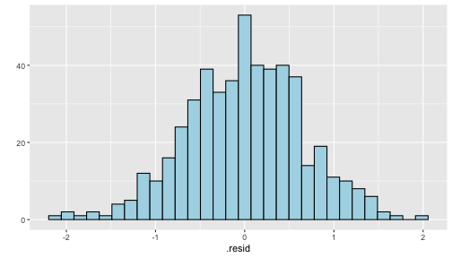<!-- --> ```r shapiro.test(regHeart_values$.resid) ``` ``` Shapiro-Wilk normality test data: regHeart_values$.resid W = 0.997, p-value = 0.4935 ``` ] .pull-right[ ```r ggplot(regHeart_values, aes(sample=.resid))+ stat_qq() + stat_qq_line() + labs(x="Theoretical Quantiles", y="Sample Quantiles") ``` 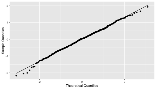<!-- --> H0: Errors are normally distributed. H1: Errors are not normally distributed. ] Decision: We do not reject H0 under 0.05 level of significance. Conclusion: We do not have enough evidence to conclude that errors are not normally distributed. --- ### Regression Diagnostics (Model adequacy checking) .blue[ 1. The relationship between the response `\(Y\)` and the predictors is linear, at least approximately. ✅ 2. The error term `\(\epsilon\)` has zero mean. ✅ 3. The error term `\(\epsilon\)` has constant variance `\(\sigma^2\)`. ✅ 4. The errors are uncorrelated. ✅ 5. The errors are normally distributed. ✅ ] .red[ Is multicollinearity a problem?] --- ## Multicollinearity Multicollinearity generally occurs when there are high correlations between two or more predictor variables. 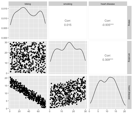<!-- --> How to Measure Multicollinearity? Next lecture. --- ### Regression Diagnostics (Model adequacy checking) .blue[ 1. The relationship between the response `\(Y\)` and the predictors is linear, at least approximately. ✅ 2. The error term `\(\epsilon\)` has zero mean. ✅ 3. The error term `\(\epsilon\)` has constant variance `\(\sigma^2\)`. ✅ 4. The errors are uncorrelated. ✅ 5. The errors are normally distributed. ✅ ] .red[ Is multicollinearity a problem? No, based on scatterplot matrix] Next week we will discuss how to measure multicollinearity. --- ## Coefficient of determination ```r summary(regHeart) ``` ``` Call: lm(formula = heart.disease ~ biking + smoking, data = heart.data) Residuals: Min 1Q Median 3Q Max -2.1789 -0.4463 0.0362 0.4422 1.9331 Coefficients: Estimate Std. Error t value Pr(>|t|) (Intercept) 14.984658 0.080137 186.99 <2e-16 *** biking -0.200133 0.001366 -146.53 <2e-16 *** smoking 0.178334 0.003539 50.39 <2e-16 *** --- Signif. codes: 0 '***' 0.001 '**' 0.01 '*' 0.05 '.' 0.1 ' ' 1 Residual standard error: 0.654 on 495 degrees of freedom Multiple R-squared: 0.9796, Adjusted R-squared: 0.9795 F-statistic: 1.19e+04 on 2 and 495 DF, p-value: < 2.2e-16 ``` .pull-left[ R-squared: `\(R^2 = 97.96\%\)` ] .pull-right[ Adjusted R-squared: `\(R^2_{adj} = 97.95\%\)` ] --- ### `\(R^2\)` and Adjusted `\(R^2_{adj}\)` - Two ways to assess the overall adequacy of the model `\(R^2\)` and Adjusted `\(R^2_{adj}\)`. - `\(R^2\)` always increases when an independent variable is added to the model, regardless of the value of the contribution of that variable. - Hence, it is difficult to judge whether an increase in `\(R^2\)` is really telling anything important. - `\(R^2_{adj}\)` will only increase on adding a variable to the model if the addition of the variable reduces the residual mean square. --- #### `\(R^2\)` and Adjusted `\(R^2_{adj}\)` - Therefore, in multiple linear regression model we prefer to use an adjusted `\(R^2_{adj}\)` statistic, defined as `$$R^2_{adj} = 1-\frac{SSE/(n-p)}{SST/(n-1)}$$` `$$\sum_{i=1}^n(y_i - \bar{y})^2=\sum_{i=1}^n(\hat{Y}_i - \bar{y})^2 + \sum_{i=1}^n(y_i - \hat{Y_i})^2$$` `$$SST = SSM + SSE$$` .pull-left[ n - total number of observations p - number of independent variables `$$MSE = \frac{SSE}{n-p}$$` ] .pull-right[ SSE - Residual (error) sum of squares SST - Total variation MSE - Residual mean square ] Coefficient of determination is a statistical measure that represents the proportion of the variance for a dependent variable that's explained by an independent variable or variables in a regression model. --- ### Interpretation of `\(R^2_{adj}\)` ``` Call: lm(formula = heart.disease ~ biking + smoking, data = heart.data) Residuals: Min 1Q Median 3Q Max -2.1789 -0.4463 0.0362 0.4422 1.9331 Coefficients: Estimate Std. Error t value Pr(>|t|) (Intercept) 14.984658 0.080137 186.99 <2e-16 *** biking -0.200133 0.001366 -146.53 <2e-16 *** smoking 0.178334 0.003539 50.39 <2e-16 *** --- Signif. codes: 0 '***' 0.001 '**' 0.01 '*' 0.05 '.' 0.1 ' ' 1 Residual standard error: 0.654 on 495 degrees of freedom Multiple R-squared: 0.9796, Adjusted R-squared: 0.9795 F-statistic: 1.19e+04 on 2 and 495 DF, p-value: < 2.2e-16 ``` Then, it means that the independent variables - biking and smoking explain 97.9% of the variation in the response variable - `heart.disease`. --- ## Interpretation of coefficients `$$Y = \beta_0 + \beta_1X_1 + \beta_2X_2+...+\beta_pX_p + \epsilon$$` .content-box-yellow[ Intercept] `\(\beta_0\)` - population mean of `\(Y\)` when all the independent variable take the value zero. If the data range of all the independent variables do not cover the value zero, do not interpret the intercept. -- .content-box-yellow[Partial regression coefficients] The parameters, `\(\beta_j, \text{ } j=1, ..p.\)` The parameter `\(\beta_j\)` represents the mean change in the response `\(Y\)` per unit change in `\(X_j\)` **when all of the remaining independent variables are held constant.** That's why `\(\beta_j, j=1, 2, ..p\)` are often called partial regression coefficients. --- Video demonstration: --- **Interpretation of coefficients (cont.)** ``` Call: lm(formula = heart.disease ~ biking + smoking, data = heart.data) Coefficients: (Intercept) biking smoking 14.9847 -0.2001 0.1783 ``` `\(\hat{\beta_0} = 14.9847\)` An estimate of population mean percentage of people who have heart disease is approximately 14.98%, when there are zero percentage of biking people and zero percentage smoking people in the town. `\(\hat{\beta_1} = -0.2001\)` This tells us that for every one percent increase in biking to work there is an associated 0.2 percent mean **decrease** in percentage of people with heart disease, when the percentage of smoking people held constant. `\(\hat{\beta_2} = 0.1783\)` For every one percent increase in the percentage of smoking people there is an associated .17 percent mean **increase** in percentage of people with heart disease, when the percentage of biking to work held constant. --- ## Next Lecture > More work - Multiple Linear Regression --- class: center, middle Acknowledgement Introduction to Linear Regression Analysis, Douglas C. Montgomery, Elizabeth A. Peck, G. Geoffrey Vining Data from https://www.scribbr.com/statistics/multiple-linear-regression/ All rights reserved by [Dr. Thiyanga S. Talagala](https://thiyanga.netlify.app/)