Recapping what we know

True linear regression model/ Population regression equation

$${\mu }_{Y|X=x}={\beta }_0+{\beta }_{1}x$$

• how the mean of $Y$ changes for given values of $X$.

• We can also write the equation in terms of the observed values of $Y$, rather than the mean. Because the individual observations for any given value of $X$ vary randomly about the mean of $Y|X$, we need to account for this random variation, or error, in the regression equation. Sample regression line

$$Y_i={\beta }_0+{\beta }_1{x}_i+{ϵ}_i,\text{i = 1, 2, 3...n}$$

Please write the assumptions of ${ϵ}_i$

Fitted regression line

$$\hat{Y}={\hat{\beta }}_0+{\hat{\beta }}_{1}x$$

Revisiting the fitted regression model

Fitted model

library(alr3) # to load the dataset

Loading required package: car

Loading required package: carData

model1 <- lm(Dheight ~ Mheight, data=heights)
model1

Call:
lm(formula = Dheight ~ Mheight, data = heights)
Coefficients:
(Intercept)      Mheight  
    29.9174       0.5417

Model summary

summary(model1)

Call:
lm(formula = Dheight ~ Mheight, data = heights)
Residuals:
   Min     1Q Median     3Q    Max 
-7.397 -1.529  0.036  1.492  9.053 
Coefficients:
            Estimate Std. Error t value Pr(>|t|)    
(Intercept) 29.91744    1.62247   18.44   <2e-16 ***
Mheight      0.54175    0.02596   20.87   <2e-16 ***
---
Signif. codes:  0 '***' 0.001 '**' 0.01 '*' 0.05 '.' 0.1 ' ' 1
Residual standard error: 2.266 on 1373 degrees of freedom
Multiple R-squared:  0.2408,    Adjusted R-squared:  0.2402 
F-statistic: 435.5 on 1 and 1373 DF,  p-value: < 2.2e-16

$R^2$ = 24.08%

• Maybe you have one or more omitted variables. It is important to consider other factors that might influence the daughter's height:

  • Father's height

  • Physical activities performed by the daughter

  • Food nutrition, etc.

• Maybe the functional form of the regression form is incorrect (so you have to add some quadratic, or cubic terms...). At the same time a transformation can be an alternative (if appropriate).

• Maybe could be the effect of a group of outlier (maybe not one...).

• A large $R^2$ does not necessarily imply that the regression model will be an accurate predictor.

• $R^2$ does not measure the appropriateness of the linear model.

• $R^2$ will often large even though $Y$ and $X$ are nonlinearly related.

[1] 0.7834839

Call:
lm(formula = carat ~ price, data = df)
Residuals:
     Min       1Q   Median       3Q      Max 
-2.91911 -0.66197 -0.07846  0.82734  2.97025 
Coefficients:
            Estimate Std. Error t value Pr(>|t|)    
(Intercept)  0.74996    0.23234   3.228   0.0017 ** 
price        0.18736    0.01501  12.481   <2e-16 ***
---
Signif. codes:  0 '***' 0.001 '**' 0.01 '*' 0.05 '.' 0.1 ' ' 1
Residual standard error: 1.137 on 98 degrees of freedom
Multiple R-squared:  0.6138,    Adjusted R-squared:  0.6099 
F-statistic: 155.8 on 1 and 98 DF,  p-value: < 2.2e-16

• $R^2$ is large even though the linear approximation is poor.

In general a good policy is to observe the scatterplot of your data

Data set

crystaldata <- data.frame(Size = c(0.08, 0.07,  1.12, 2.01, 4.43, 
                                   4.98, 4.92, 7.18, 
                                   5.57, 8.40, 8.81, 10.81, 11.61, 10.12, 13.12, 15.04, 0.075, 0.075,  1.13, 2.02, 4.45, 
                                   4.99, 4.95, 7.28, 
                                   5.67, 8.40, 8.51, 10.82, 11.62, 10.13, 13.22, 15.03),
  Time= c(2, 2, 4, 4,6, 8, 10, 12, 14, 16, 18, 20, 20, 24, 26, 28, 2, 2, 4, 4,6, 8, 10, 12, 14, 16, 18, 20, 20, 24, 26, 28))
crystaldata

     Size Time
1   0.080    2
2   0.070    2
3   1.120    4
4   2.010    4
5   4.430    6
6   4.980    8
7   4.920   10
8   7.180   12
9   5.570   14
10  8.400   16
11  8.810   18
12 10.810   20
13 11.610   20
14 10.120   24
15 13.120   26
16 15.040   28
17  0.075    2
18  0.075    2
19  1.130    4
20  2.020    4
21  4.450    6
22  4.990    8
23  4.950   10
24  7.280   12
25  5.670   14
26  8.400   16
27  8.510   18
28 10.820   20
29 11.620   20
30 10.130   24
31 13.220   26
32 15.030   28

scatterplot

ggplot(crystaldata, aes(x=Time, y = Size)) + geom_point()

cor(crystaldata$Time, crystaldata$Size)

[1] 0.9741803

Fit a simple linear regression model

mod1 <- lm(Size ~ Time, data=crystaldata)
mod1

Call:
lm(formula = Size ~ Time, data = crystaldata)
Coefficients:
(Intercept)         Time  
    -0.1982       0.5210

Visualise the model

ggplot(crystaldata, aes(y=Size, x=Time))+geom_point(alpha=0.5) +
  geom_abline(intercept = -0.21, slope = 0.52, colour="forestgreen", lwd=2) +
            theme(aspect.ratio = 1)

Questions

1. How well does this equation fit the data?

2. Are any of the basic assumptions violated?

summary(mod1)

Call:
lm(formula = Size ~ Time, data = crystaldata)
Residuals:
    Min      1Q  Median      3Q     Max 
-2.1855 -0.7643  0.0313  0.7405  1.5223 
Coefficients:
            Estimate Std. Error t value Pr(>|t|)    
(Intercept) -0.19821    0.34838  -0.569    0.574    
Time         0.52099    0.02204  23.634   <2e-16 ***
---
Signif. codes:  0 '***' 0.001 '**' 0.01 '*' 0.05 '.' 0.1 ' ' 1
Residual standard error: 1.05 on 30 degrees of freedom
Multiple R-squared:  0.949,    Adjusted R-squared:  0.9473 
F-statistic: 558.5 on 1 and 30 DF,  p-value: < 2.2e-16

Coefficient of determination

Call:
lm(formula = Size ~ Time, data = crystaldata)
Residuals:
    Min      1Q  Median      3Q     Max 
-2.1855 -0.7643  0.0313  0.7405  1.5223 
Coefficients:
            Estimate Std. Error t value Pr(>|t|)    
(Intercept) -0.19821    0.34838  -0.569    0.574    
Time         0.52099    0.02204  23.634   <2e-16 ***
---
Signif. codes:  0 '***' 0.001 '**' 0.01 '*' 0.05 '.' 0.1 ' ' 1
Residual standard error: 1.05 on 30 degrees of freedom
Multiple R-squared:  0.949,    Adjusted R-squared:  0.9473 
F-statistic: 558.5 on 1 and 30 DF,  p-value: < 2.2e-16

• 94.5% of the variability in size is accounted by the regression model.

or

• 94.5% of the variation in size is explained by the number of hours it takes crystal to grow.

Are any of the basic assumptions violated?

mod1

Call:
lm(formula = Size ~ Time, data = crystaldata)
Coefficients:
(Intercept)         Time  
    -0.1982       0.5210

Compute Residuals and Fitted values

library(broom)

Warning: package 'broom' was built under R version 4.1.2

mod1_fitresid <- augment(mod1)
mod1_fitresid

# A tibble: 32 × 8
    Size  Time .fitted  .resid   .hat .sigma  .cooksd .std.resid
   <dbl> <dbl>   <dbl>   <dbl>  <dbl>  <dbl>    <dbl>      <dbl>
 1  0.08     2   0.844 -0.764  0.0883   1.06 0.0281      -0.762 
 2  0.07     2   0.844 -0.774  0.0883   1.06 0.0289      -0.772 
 3  1.12     4   1.89  -0.766  0.0700   1.06 0.0215      -0.756 
 4  2.01     4   1.89   0.124  0.0700   1.07 0.000567     0.123 
 5  4.43     6   2.93   1.50   0.0552   1.03 0.0634       1.47  
 6  4.98     8   3.97   1.01   0.0440   1.05 0.0223       0.984 
 7  4.92    10   5.01  -0.0917 0.0363   1.07 0.000149    -0.0890
 8  7.18    12   6.05   1.13   0.0321   1.05 0.0197       1.09  
 9  5.57    14   7.10  -1.53   0.0314   1.03 0.0354      -1.48  
10  8.4     16   8.14   0.262  0.0343   1.07 0.00115      0.254 
# … with 22 more rows

1) The relationship between the response $Y$ and the regressors is linear, at least approximately.

Plot of residuals vs fitted values and Plot of residuals vs predictor

2) The error term $ϵ$ has zero mean.

3) The error term $ϵ$ has constant variance ${\sigma }^2$.

Residuals vs Fitted

4) The error are uncorrelated.

5) The errors are normally distributed.

ggplot(mod1_fitresid, 
       aes(x=.resid))+
  geom_histogram(colour="white")+ggtitle("Distribution of Residuals")

ggplot(mod1_fitresid, 
       aes(sample=.resid))+
  stat_qq() + stat_qq_line()+labs(x="Theoretical Quantiles", y="Sample Quantiles")

shapiro.test(mod1_fitresid$.resid)

    Shapiro-Wilk normality test
data:  mod1_fitresid$.resid
W = 0.95397, p-value = 0.1867

Interpretations

$${\mu }_{Y|X=x}={\beta }_0+{\beta }_{1}x$$

Slope:

Increase in the mean response for every one unit increase in the explanatory variable.

Intercept:

Mean response when the explanatory variable equals 0

mod1

Call:
lm(formula = Size ~ Time, data = crystaldata)
Coefficients:
(Intercept)         Time  
    -0.1982       0.5210

Interpret slope and intercept

Nonsensical intercept interpretation

• Sometimes it doesn't make sense to interpret the intercept: when?

  • $X$ can never realistically take the value of zero, then the intercept is meaningless.

  • The intercept is negative even though the response can take only positive values.

• The intercept helps the line fit the data as closely as possible.

• It is fine to have a regression model with nonsensical intercept if it helps the model give better overall prediction accuracy.

Hypothesis testing - Intercept

$H_0:{\beta }_1=0$

$H_1:{\beta }_1\ne 0$

summary(mod1)

Call:
lm(formula = Size ~ Time, data = crystaldata)
Residuals:
    Min      1Q  Median      3Q     Max 
-2.1855 -0.7643  0.0313  0.7405  1.5223 
Coefficients:
            Estimate Std. Error t value Pr(>|t|)    
(Intercept) -0.19821    0.34838  -0.569    0.574    
Time         0.52099    0.02204  23.634   <2e-16 ***
---
Signif. codes:  0 '***' 0.001 '**' 0.01 '*' 0.05 '.' 0.1 ' ' 1
Residual standard error: 1.05 on 30 degrees of freedom
Multiple R-squared:  0.949,    Adjusted R-squared:  0.9473 
F-statistic: 558.5 on 1 and 30 DF,  p-value: < 2.2e-16

Situations where $H_0:{\beta }_1=0$ is not rejected.

In-class

Situations where $H_0:{\beta }_1=0$ is rejected.

In-class

Confidence Interval on ${\beta }_0$ and ${\beta }_1$

• Confidence intervals ${\beta }_0$

$$[\widehat{{\beta }_0}-t_{\alpha /2,n-2}se(\widehat{{\beta }_0}),\widehat{{\beta }_0}+t_{\alpha /2,n-2}se(\widehat{{\beta }_0}\left)\right]$$

• Confidence intervals ${\beta }_1$

$$[\widehat{{\beta }_1}-t_{\alpha /2,n-2}se(\widehat{{\beta }_1}),\widehat{{\beta }_1}+t_{\alpha /2,n-2}se(\widehat{{\beta }_1}\left)\right]$$

t-distribution

$t_{0.025,30}$

qt(0.975, df=30)

[1] 2.042272

qt(0.025, df=30)

[1] -2.042272

summary(mod1)

Call:
lm(formula = Size ~ Time, data = crystaldata)
Residuals:
    Min      1Q  Median      3Q     Max 
-2.1855 -0.7643  0.0313  0.7405  1.5223 
Coefficients:
            Estimate Std. Error t value Pr(>|t|)    
(Intercept) -0.19821    0.34838  -0.569    0.574    
Time         0.52099    0.02204  23.634   <2e-16 ***
---
Signif. codes:  0 '***' 0.001 '**' 0.01 '*' 0.05 '.' 0.1 ' ' 1
Residual standard error: 1.05 on 30 degrees of freedom
Multiple R-squared:  0.949,    Adjusted R-squared:  0.9473 
F-statistic: 558.5 on 1 and 30 DF,  p-value: < 2.2e-16

Compute confidence intervals on slope and intercept

Confidence Interval on ${\beta }_0$ and ${\beta }_1$ - Interpretation

• Confidence intervals ${\beta }_0$

$$[\widehat{{\beta }_0}-t_{\alpha /2,n-2}se(\widehat{{\beta }_0}),\widehat{{\beta }_0}+t_{\alpha /2,n-2}se(\widehat{{\beta }_0}\left)\right]$$

• Confidence intervals ${\beta }_1$

$$[\widehat{{\beta }_1}-t_{\alpha /2,n-2}se(\widehat{{\beta }_1}),\widehat{{\beta }_1}+t_{\alpha /2,n-2}se(\widehat{{\beta }_1}\left)\right]$$

Frequency interpretation:

If we were to take repeated samples of the same size at the same $X$ levels and construct, for example, $95\%$ confidence intervals on the slope for each sample, then $95\%$ of those intervals will contain the true value ${\beta }_1$.

We therefore have considerable confidence that the observed interval, here (04792, 0.5608), covers the true ${\beta }_1$. The measure of confidence is .95. Here, .95 is called the confidence coefficient.

In general, the larger the confidence coefficient $(1-\alpha )$ is, the wider the confidence interval.

page 375, Mood and Graybill, Introduction to the theory of statistics

Analysis of variance - ANOVA

• We may also use ANOVA to test the significance of regression.

• The idea behind the ANOVA is that the variation in the response variable (referred to as the total variation - SST) is partitioned into two parts:

i. how much of the variation is explained by the regression model (referred to as the variable name in the R output) - SSM (Model sum of squares)

ii. how much of the variation is left unexplained by the regression model (called the “Residual” or “Error”) - SSE (Residual or error sum of squares).

$$\sum _{i=1}^n(y_i-\overline{y}{)}^2=\sum _{i=1}^n({\hat{Y}}_i-\overline{y}{)}^2+\sum _{i=1}^n(y_i-\widehat{Y_i}{)}^2$$

$$SST=SSM+SSE$$

Degrees of component

$$d{f}_T=d{f}_M+d{f}_E$$ $$n-1=1+(n-2)$$

ANOVA - F test

$$F=\frac{SSM/d{f}_M}{SSE/d{f}_E}=\frac{M{S}_M}{M{S}_E}$$

$$E\left(M{S}_E\right)={\sigma }^2$$

ANOVA - Hypothesis

$$H_0:{\beta }_1=0$$ $$H_1:{\beta }_1\ne 0$$

• In simple linear regression t-test is equivalent to the F test.

• The real usefulness of the analysis of variance is in multiple regression models.

anova(mod1)

Analysis of Variance Table
Response: Size
          Df Sum Sq Mean Sq F value    Pr(>F)    
Time       1 615.46  615.46  558.55 < 2.2e-16 ***
Residuals 30  33.06    1.10                      
---
Signif. codes:  0 '***' 0.001 '**' 0.01 '*' 0.05 '.' 0.1 ' ' 1

summary(mod1)

Call:
lm(formula = Size ~ Time, data = crystaldata)
Residuals:
    Min      1Q  Median      3Q     Max 
-2.1855 -0.7643  0.0313  0.7405  1.5223 
Coefficients:
            Estimate Std. Error t value Pr(>|t|)    
(Intercept) -0.19821    0.34838  -0.569    0.574    
Time         0.52099    0.02204  23.634   <2e-16 ***
---
Signif. codes:  0 '***' 0.001 '**' 0.01 '*' 0.05 '.' 0.1 ' ' 1
Residual standard error: 1.05 on 30 degrees of freedom
Multiple R-squared:  0.949,    Adjusted R-squared:  0.9473 
F-statistic: 558.5 on 1 and 30 DF,  p-value: < 2.2e-16

Regression through the origin (No intercept)

• Appropriate in analysing data from chemical and other manufacturing processes.

• Do not misuse the no-intercept model: where the data lie in a region of $x$-space remote from the origin.

• Scatterplot sometimes helps in deciding whether or not to fit the no-intercept model.

How to select the model: Fit both models (with intercept and without intercept) and choose between them based on the quality of the fit.

mod2 <- lm(Size ~ Time -1, data=crystaldata)
mod2

Call:
lm(formula = Size ~ Time - 1, data = crystaldata)
Coefficients:
  Time  
0.5104

summary(mod2)

Call:
lm(formula = Size ~ Time - 1, data = crystaldata)
Residuals:
     Min       1Q   Median       3Q      Max 
-2.12895 -0.92631 -0.04059  0.78642  1.41254 
Coefficients:
     Estimate Std. Error t value Pr(>|t|)    
Time  0.51037    0.01161   43.95   <2e-16 ***
---
Signif. codes:  0 '***' 0.001 '**' 0.01 '*' 0.05 '.' 0.1 ' ' 1
Residual standard error: 1.038 on 31 degrees of freedom
Multiple R-squared:  0.9842,    Adjusted R-squared:  0.9837 
F-statistic:  1931 on 1 and 31 DF,  p-value: < 2.2e-16

ggplot(crystaldata, aes(y=Size, x=Time))+geom_point(alpha=0.5) +
  geom_abline(intercept = -0.21, slope = 0.52, colour="forestgreen", lwd=2) +
            theme(aspect.ratio = 1)

ggplot(crystaldata, aes(y=Size, x=Time))+geom_point(alpha=0.5) +
  geom_abline(intercept = 0, slope = 0.51, colour="red", lwd=2) +
            theme(aspect.ratio = 1)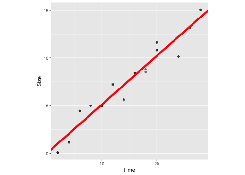

Perform the residual analysis on the new model before using it.

test <- data.frame(Time = c(2, 2, 6, 6, 8, 20, 26))
test

  Time
1    2
2    2
3    6
4    6
5    8
6   20
7   26

predict(mod2, newdata=test, interval="predict")

        fit        lwr       upr
1  1.020746 -1.0972070  3.138699
2  1.020746 -1.0972070  3.138699
3  3.062237  0.9400507  5.184424
4  3.062237  0.9400507  5.184424
5  4.082983  1.9570988  6.208867
6 10.207457  8.0376929 12.377222
7 13.269695 11.0645387 15.474851

Next Lecture

Multiple linear regression