class: center, middle, inverse, title-slide # STA 506 2.0 Linear Regression Analysis ## Lecture 2: Simple Linear Regression ### Dr Thiyanga S. Talagala ### Lesson 2 --- ## Recap: correlation 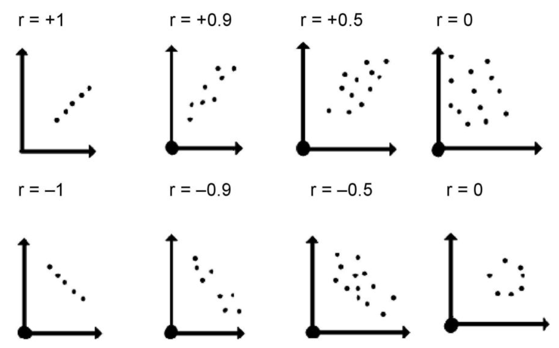 --- ## Recap: correlation (cont.) .pull-left[  ] .pull-right[ |value |interpretation | |:-------------|:---------------------| |-1 |Perfect negative | |(-1, -0.75) |Strong negative | |(-0.75, -0.5) |Moderate negative | |(-0.5, -0.25) |Weak negative | |(-0.25, 0.25) |No linear association | |(0.25, 0.5) |Weak positive | |(0.5, 0.75) |Moderate positive | |(0.75, 1) |Strong positive | |1 |Perfect positive | ] --- ## Recap: Terminologies - Response variable: dependent variable - Explanatory variables: independent variables, predictors, regressor variables, features (in Machine Learning) > Response variable = Model function + Random Error - Parameter - Statistic - Estimator - Estimate [Read my blogpost](https://thiyanga.netlify.app/post/statterms1/) --- # In-class --- # In-class --- # Simple Linear Regression **Simple** - single regressor **Linear** - parameters enter in a linear fashion. --- # Meaning of Linear Model | What about this? `$$Y = \beta_0 + \beta_1x_1 + \beta_{2}x_2 + \epsilon$$` -- | Linear or nonlinear? `$$Y = \beta_0 + \beta_1x + \beta_{2}x^2 + \epsilon$$` <!--While the independent variable is squared, the model is still linear in the parameters. Linear models can also contain log terms and inverse terms to follow different kinds of curves and yet continue to be linear in the parameters.--> -- | Linear or nonlinear? `$$Y = \beta_0e^{\beta_1x} + \epsilon$$` -- What about this? `$$Y = \alpha X_1^\beta X_2^\gamma X_3^\delta e^\epsilon$$` --- **True relationship between X and Y in the population** `$$Y = f(X) + \epsilon$$` **If `\(f\)` is approximated by a linear function** `$$Y = \beta_0 + \beta_1X + \epsilon$$` The error terms are normally distributed with mean `\(0\)` and variance `\(\sigma^2\)`. Then the mean response, `\(Y\)`, at any value of the `\(X\)` is `$$E(Y|X=x_i) = E(\beta_0 + \beta_1x_i + \epsilon)=\beta_0+\beta_1x_i$$` For a single unit `\((y_i, x_i)\)` `$$y_i = \beta_0 + \beta_1x_i+\epsilon_i \text{ where } \epsilon_i \sim N(0, \sigma^2)$$` We use sample values `\((y_i, x_i)\)` where `\(i=1, 2, ...n\)` to estimate `\(\beta_0\)` and `\(\beta_1\)`. The fitted regression model is `$$\hat{Y_i} = \hat{\beta}_0 + \hat{\beta}_1x_i$$` --- 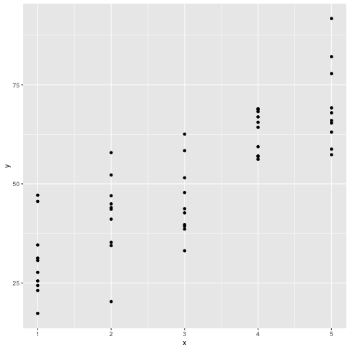<!-- --> --- ## Population mean 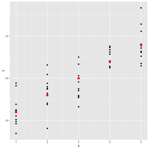<!-- --> --- ## Population mean (red) and sample mean (green) 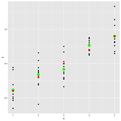<!-- --> --- ## Population Regression `$$E(Y|X=x_i) = \beta_0+\beta_1x_i$$` 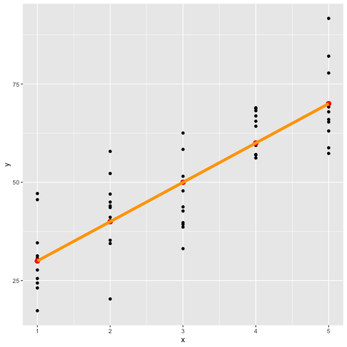<!-- --> --- ## Population regression line and fitted regression line 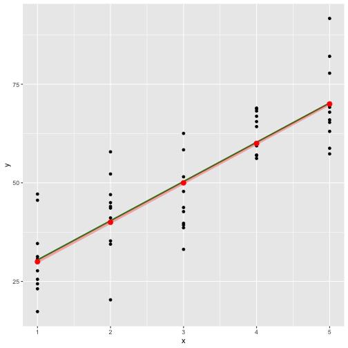<!-- --> --- ## Normal distribution .pull-left[ 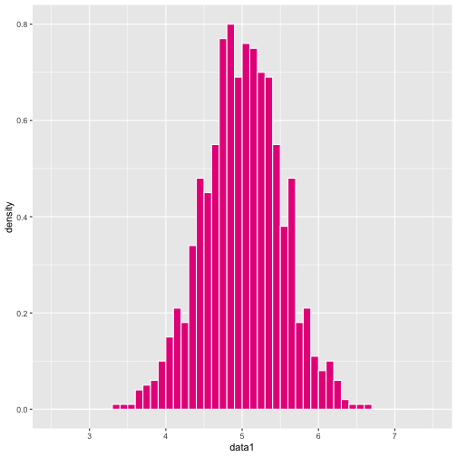<!-- --> ``` [1] 5.008403 ``` ] .pull-left[ 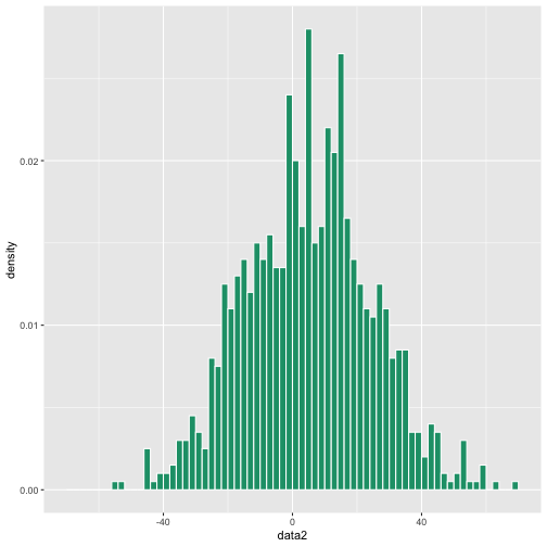<!-- --> ``` [1] 5.082935 ``` ] --- ## Normal distribution .pull-left[ 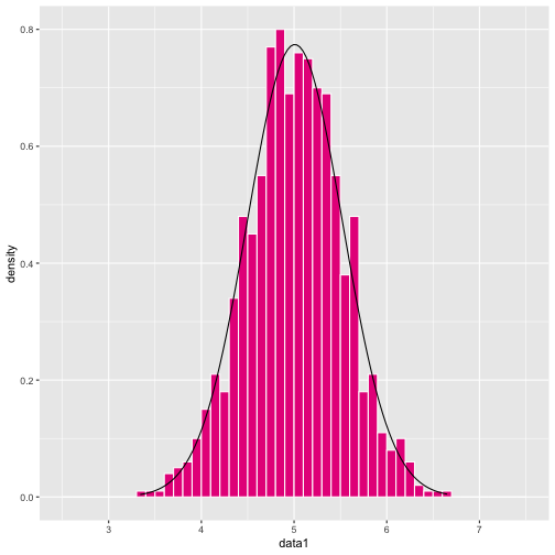<!-- --> ] .pull-left[ 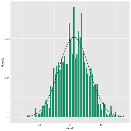<!-- --> ] --- ### Normal distribution 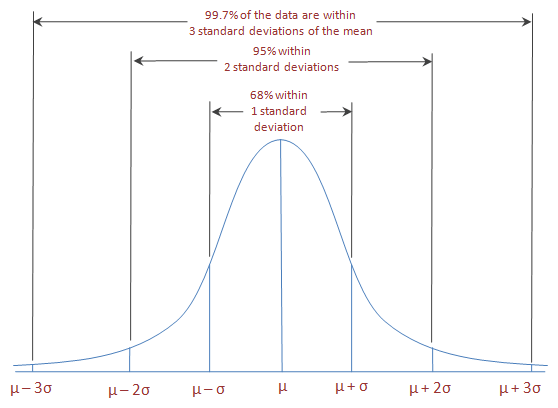 From: https://towardsdatascience.com/do-my-data-follow-a-normal-distribution-fb411ae7d832 --- ### Normal distribution 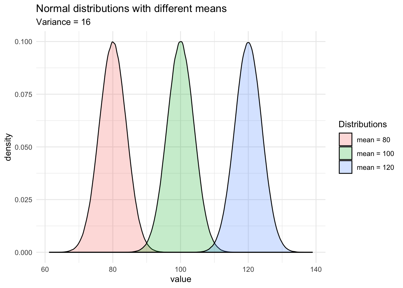 From: https://towardsdatascience.com/do-my-data-follow-a-normal-distribution-fb411ae7d832 --- ### Normal distribution  From: https://towardsdatascience.com/do-my-data-follow-a-normal-distribution-fb411ae7d832 --- class: duke-orange, center, middle ## Buckle up! ### Let's walk through the steps. --- ## In-class **True relationship between X and Y in the population** `$$Y = f(X) + \epsilon$$` > --- ## In-class **True relationship between X and Y in the population** `$$Y = f(X) + \epsilon$$` Example: Suppose you want to model daughters' height as a function of mothers' height. Do you think an exact (deterministic) relationship exists between these two variables? --- ## In-class **True relationship between X and Y in the population** `$$Y = f(X) + \epsilon$$` Example: Suppose you want to model daughters' height as a function of mothers' height. Do you think an exact (deterministic) relationship exists between these two variables? > Why? --- ## In-class **True relationship between X and Y in the population** `$$Y = f(X) + \epsilon$$` Example: Suppose you want to model daughters' height as a function of mothers' height. Do you think an exact (deterministic) relationship exists between these two variables? 1. Daughters' height may depend on many other variables than Mothers' height. --- ## In-class **True relationship between X and Y in the population** `$$Y = f(X) + \epsilon$$` Example: Suppose you want to model daughters' height as a function of mothers' height. Do you think an exact (deterministic) relationship exists between these two variables? 1. Daughters' height may depend on many other variables than Mothers' height. 2. Even if many variables are included in the model, it is unlikely that we can predict the daughter's height exactly. Why? --- ## In-class **True relationship between X and Y in the population** `$$Y = f(X) + \epsilon$$` Example: Suppose you want to model daughters' height as a function of mothers' height. Do you think an exact (deterministic) relationship exists between these two variables? 1. Daughters' height may depend on many other variables than Mothers' height. 2. Even if many variables are included in the model, it is unlikely that we can predict the daughter's height exactly. Why? There will almost certainly be some variations in the model predictions that cannot be modelled, or explained. These unexplained variances are assumed to be caused by the unexplainable random phenomena, so they can be referred to as random error. --- ## In-class --- ## In-class: Population Regression Line **True relationship between X and Y in the population** `$$Y = f(X) + \epsilon$$` **If `\(f\)` is approximated by a linear function** `$$Y = \beta_0 + \beta_1X + \epsilon$$` The error terms are normally distributed with mean `\(0\)` and variance `\(\sigma^2\)`. Then the mean response, `\(Y\)`, at any value of the `\(X\)` is `$$E(Y|X=x_i) = E(\beta_0 + \beta_1x_i + \epsilon)=\beta_0+\beta_1x_i$$` ---  ---  source: http://digfir-published.macmillanusa.com/psbe4e/psbe4e_ch10_2.html ---  source: https://tex.stackexchange.com/questions/347744/assumptions-for-simple-linear-regression --- ## In-class: Population Regression Line `$$E(Y|X=x_i) = E(\beta_0 + \beta_1x_i + \epsilon)=\beta_0+\beta_1x_i$$` For a single unit `\((y_i, x_i)\)` `$$y_i = \beta_0 + \beta_1x_i+\epsilon_i \text{ where } \epsilon_i \sim N(0, \sigma^2)$$` --- ## Take a sample: The fitted regression line is `$$\hat{Y_i} = \hat{\beta}_0 + \hat{\beta}_1x_i$$` --- ## Our example Dashboard: https://statisticsmart.shinyapps.io/SimpleLinearRegression/ 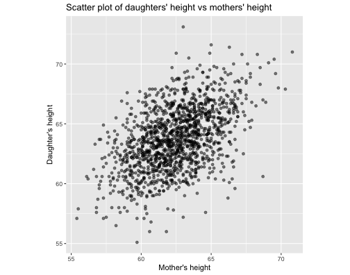<!-- --> --- ## Our example (0.52, 30.7) Dashboard: https://statisticsmart.shinyapps.io/SimpleLinearRegression/ <!-- --> --- ## Our example (0.582, 28.5) Dashboard: https://statisticsmart.shinyapps.io/SimpleLinearRegression/ <!-- --> --- ## Our example (0.5, 32.5) Dashboard: https://statisticsmart.shinyapps.io/SimpleLinearRegression/ 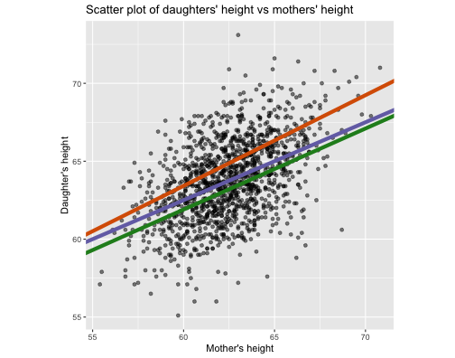<!-- --> ## Which is the best? --- ## Which is the best? .pull-left[ 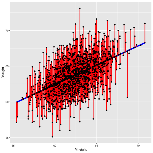<!-- --> ] .pull-right[ Sum of squares of **Residuals** `$$SSR=e_1^2+e_2^2+...+e_n^2$$` ] --- ## Evaluating your answers: Fitted values .pull-left[ <!-- --> ] .pull-right[ Dheight = 30.7 + 0.52Mheight ```r df <- alr3::heights df$fitted <- 30.7 + (0.52*df$M) head(df,10) ``` ``` Mheight Dheight fitted 1 59.7 55.1 61.744 2 58.2 56.5 60.964 3 60.6 56.0 62.212 4 60.7 56.8 62.264 5 61.8 56.0 62.836 6 55.5 57.9 59.560 7 55.4 57.1 59.508 8 56.8 57.6 60.236 9 57.5 57.2 60.600 10 57.3 57.1 60.496 ``` First fitted value: 30.7 + (0.52 * 59.7) = 61.744 ] --- ## Evaluating your answers .pull-left[ 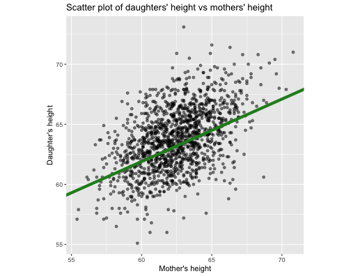<!-- --> Sum of squares of **Residuals** `$$SSR=e_1^2+e_2^2+...+e_n^2$$` ] .pull-right[ Dheight = 30.7 + 0.52Mheight ``` Mheight Dheight fitted resid_squared 1 59.7 55.1 61.744 44.142736 2 58.2 56.5 60.964 19.927296 3 60.6 56.0 62.212 38.588944 4 60.7 56.8 62.264 29.855296 5 61.8 56.0 62.836 46.730896 6 55.5 57.9 59.560 2.755600 7 55.4 57.1 59.508 5.798464 8 56.8 57.6 60.236 6.948496 9 57.5 57.2 60.600 11.560000 10 57.3 57.1 60.496 11.532816 ``` ``` [1] 7511.118 ``` SSR: 7511.118 ] --- ## Evaluating your answers Dashboard: https://statisticsmart.shinyapps.io/SimpleLinearRegression/ .pull-left[ <!-- --> ] .pull-right[ - Green: 7511.118 (0.52, 30.7) - Orange: 8717.41 (0.582, 28.5) - Purple: 7066.075 (0.5, 32.5) ] --- ### How to estimate `\(\beta_0\)` and `\(\beta_1\)`? Sum of squares of Residuals `$$SSR=e_1^2+e_2^2+...+e_n^2$$` **Observed value** `\(y_i\)` **Fitted value** `\(\hat{Y_i}\)` `\(\hat{Y_i} = \hat{\beta}_0 + \hat{\beta}_1x_i\)` **Residual** `\(e_i = y_i - \hat{Y_i}\)` The least-squares regression approach chooses coefficients `\(\hat{\beta}_0\)` and `\(\hat{\beta}_1\)` to minimize `\(SSR\)`. --- ### Least-squares Estimation of the Parameters `$$y_i = \beta_0 + \beta_1x_i + \epsilon_i \text{, i =1, 2, 3, ...n .}$$` The least squares criterion is `$$S(\beta_0, \beta_1) = \sum_{i=1}^n (y_i - \beta_0 - \beta_1x_i)^2.$$` --- ### Least-squares Estimation of the Parameters (cont.) The least squares criterion is `$$S(\beta_0, \beta_1) = \sum_{i=1}^n (y_i - \beta_0 - \beta_1x_i)^2.$$` The least-squares estimators of `\(\beta_0\)` and `\(\beta_1\)`, say `\(\hat{\beta_0}\)` and `\(\hat{\beta_1},\)` must satisfy `$$\frac{\partial S}{\partial \beta_0}|_{\hat{\beta_0}, \hat{\beta_1}} = -2\sum_{i=1}^{n}(y_i - \hat{\beta_0} - \hat{\beta_1}x_i) = 0$$` and `$$\frac{\partial S}{\partial \beta_1}|_{\hat{\beta_0}, \hat{\beta_1}} = -2\sum_{i=1}^{n}(y_i - \hat{\beta_0} - \hat{\beta_1}x_i)x_i = 0.$$` --- ### Least-squares Estimation of the Parameters (cont.) Simplifying the two equations yields `$$n\hat{\beta_0}+\hat{\beta_1}\sum_{i=1}^nx_i=\sum_{i=1}^ny_i,$$` `$$\hat{\beta_0}\sum_{i=1}^nx_i+\hat{\beta_1}\sum_{i=1}^nx^2_i=\sum_{i=1}^ny_ix_i.$$` These are called **least-squares normal equations**. --- ## Least-squares Estimation of the Parameters (cont.) `$$n\hat{\beta_0}+\hat{\beta_1}\sum_{i=1}^nx_i=\sum_{i=1}^ny_i,$$` `$$\hat{\beta_0}\sum_{i=1}^nx_i+\hat{\beta_1}\sum_{i=1}^nx^2_i=\sum_{i=1}^ny_ix_i.$$` The solution to the normal equation is `$$\hat{\beta_0} = \bar{y} - \hat{\beta_1}\bar{x},$$` and `$$\hat{\beta_1} = \frac{\sum_{i=1}^ny_ix_i - \frac{\sum_{i=1}^ny_i\sum_{i=1}^nx_i}{n}}{\sum_{i=1}^nx_i^2 - \frac{(\sum_{i=1}^nx_i)^2}{n}}.$$` The fitted simple linear regression model is then `$$\hat{Y} = \hat{\beta_0} + \hat{\beta}_1x$$` --- ## Least-squares fit > Try this with R ```r library(alr3) # to load the dataset model1 <- lm(Dheight ~ Mheight, data=heights) model1 ``` ``` Call: lm(formula = Dheight ~ Mheight, data = heights) Coefficients: (Intercept) Mheight 29.9174 0.5417 ``` --- ## Least-squares fit and your guesses <!-- --> ```r fit <- 0.5417 * df$Mheight + 29.9174 sum((df$Dheight - fit)^2) ``` ``` [1] 7051.97 ``` --- # Least square fit and your guesses .pull-left[ 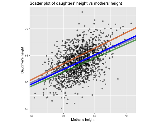<!-- --> ] .pull-right[ - Green: 7511.118 (0.52, 30.7) - Orange: 8717.41 (0.582, 28.5) - Purple: 7066.075 (0.5, 32.5) - Blue: **7051.97** (0.541, 29.9174) ] --- ## Try this with R ```r library(alr3) # to load the dataset model1 <- lm(Dheight ~ Mheight, data=heights) model1 ``` ```r summary(model1) ``` ``` Call: lm(formula = Dheight ~ Mheight, data = heights) Residuals: Min 1Q Median 3Q Max -7.397 -1.529 0.036 1.492 9.053 Coefficients: Estimate Std. Error t value Pr(>|t|) (Intercept) 29.91744 1.62247 18.44 <2e-16 *** Mheight 0.54175 0.02596 20.87 <2e-16 *** --- Signif. codes: 0 '***' 0.001 '**' 0.01 '*' 0.05 '.' 0.1 ' ' 1 Residual standard error: 2.266 on 1373 degrees of freedom Multiple R-squared: 0.2408, Adjusted R-squared: 0.2402 F-statistic: 435.5 on 1 and 1373 DF, p-value: < 2.2e-16 ``` --- ## Visualise the model: Try with R ```r ggplot(data=heights, aes(x=Mheight, y=Dheight)) + geom_point(alpha=0.5) + geom_smooth(method="lm", se=FALSE, col="blue", lwd=2) + theme(aspect.ratio = 1) ``` 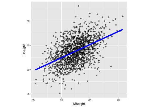<!-- --> --- ## Least squares regression line .pull-left[ 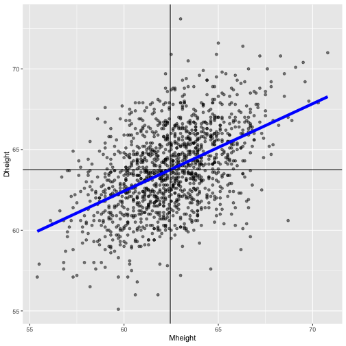<!-- --> ] .pull-right[ ```r summary(alr3::heights) ``` ``` Mheight Dheight Min. :55.40 Min. :55.10 1st Qu.:60.80 1st Qu.:62.00 Median :62.40 Median :63.60 Mean :62.45 Mean :63.75 3rd Qu.:63.90 3rd Qu.:65.60 Max. :70.80 Max. :73.10 ``` ] The LSRL passes through the point ( `\(\bar{x}\)`, `\(\bar{y}\)`), that is (sample mean of `\(x\)`, sample mean of `\(y\)`) --- ## Least squares regression line .pull-left[ 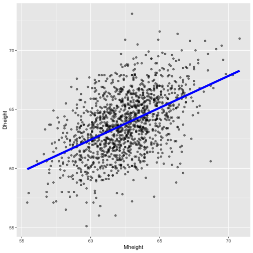<!-- --> ] .pull-right[ The least squares regression line doesn't match the population regression line perfectly, but it is a pretty good estimate. And, of course, we'd get a different least squares regression line if we took another (different) sample. ] --- background-image: url('reg7.PNG') background-position: center background-size: contain --- ## Extrapolation: beyond the scope of the model. <!-- --> --- ## Next Lecture > More work - Simple Linear Regression, Residual Analysis, Predictions --- class: center, middle All rights reserved by [Dr. Thiyanga S. Talagala](https://thiyanga.netlify.app/)