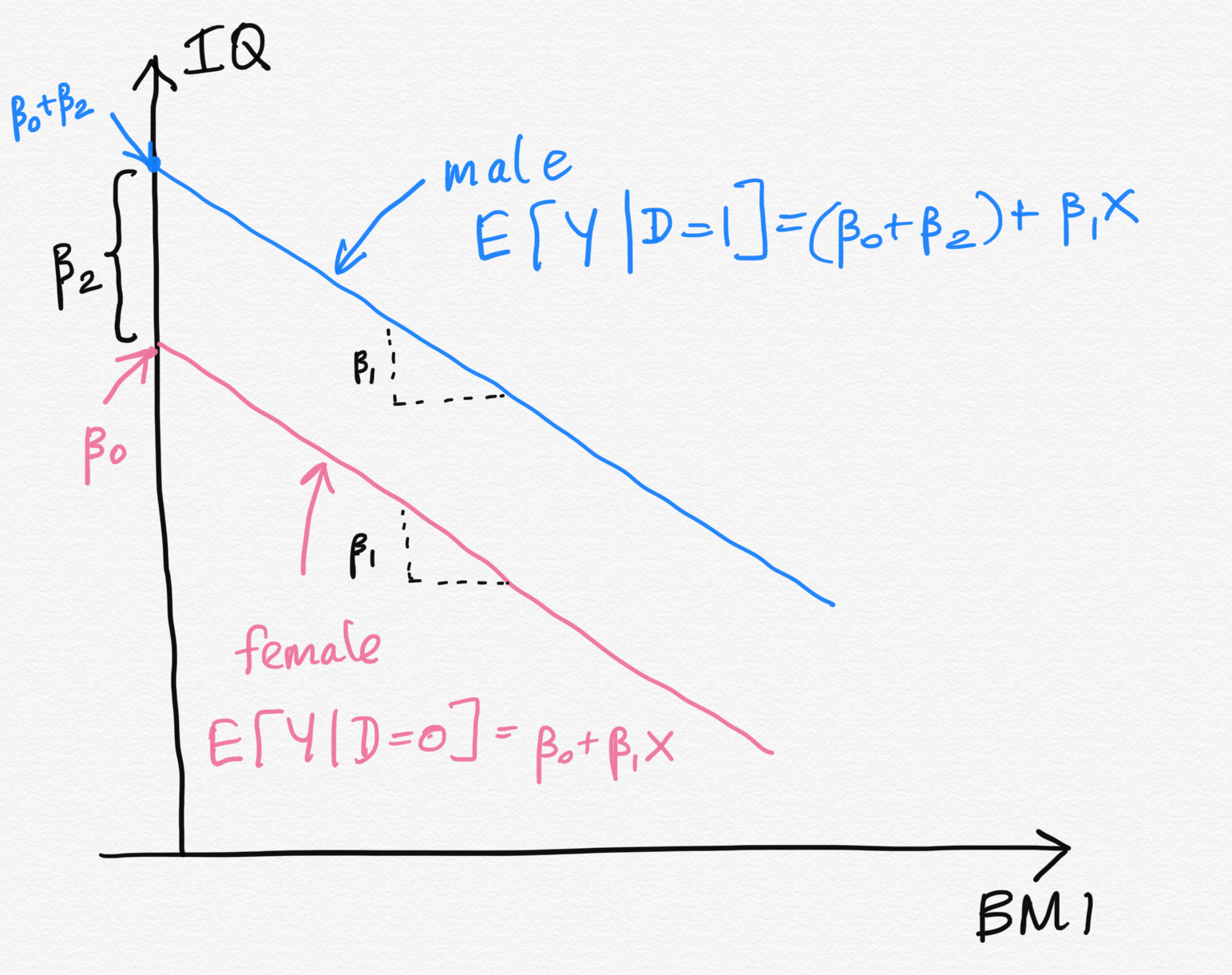
class: center, middle, inverse, title-slide # STA 506 2.0 Linear Regression Analysis ## Lecture 12-ii: Indicator Variables ### Dr Thiyanga S. Talagala --- ## Introduction - All the independent variables we have considered up to this point have been measured on a continuous scale. - Regression analysis can be generalized to incorporate qualitative variables. - Examples of qualitative variables: - Gender (male, female) - Smoking status (smoker, nonsmoker) - Employment status (full-time, part-time, unemployed) - BMI (underweight, normal, overweight, obese) - Categorical variables can be incorporated into regression through **indicator variables**. - Sometimes indicator variables are called **dummy variable.** --- ## Creating dummy variables ``` IQ Gender BMI 1 10 Male 20.2 2 20 Male 20.5 3 100 Male 18.5 4 98 Male 25.0 5 100 Female 24.9 6 11 Female 31.0 7 50 Female 18.5 8 70 Female 20.0 ``` Indicator variable for `Gender` `$$D_i = \left\{ \begin{array}\\ 1 & \mbox{if male} \\ 0 & \mbox{if female} \end{array} \right.$$` The choice of 0 and 1 to identify the levels of a qualitative variable is arbitrary. --- ## Regression equation .pull-left[ ``` IQ Gender BMI D 1 10 Male 20.2 1 2 20 Male 20.5 1 3 100 Male 18.5 1 4 98 Male 25.0 1 5 100 Female 24.9 0 6 11 Female 31.0 0 7 50 Female 18.5 0 8 70 Female 20.0 0 ``` ] .pull-right[ Indicator variable for `Gender` `$$D_i = \left\{ \begin{array}\\ 1 & \mbox{if male} \\ 0 & \mbox{if female} \end{array} \right.$$` ] Regression equation `$$y_i = \beta_0 + \beta_1 x_i + \beta_2D_i + \epsilon_i,$$` where `\(x\)` represents the variable `BMI`. --- ## Regression equation (cont.) `$$y_i = \beta_0 + \beta_1 x_i + \beta_2D_i + \epsilon_i,$$` where `\(x\)` represents the variable `BMI`. ### Regression equation for **males**, `\(D_i = 1\)` `$$y_i = \beta_0 + \beta_1 x_i + \beta_2 + \epsilon_i,$$` `$$y_i = (\beta_0 + \beta_2) + \beta_1 x_i + \epsilon_i,$$` - Thus the relationship between **IQ score** and **BMI** for **males** is a straight line with intercept `\(\beta_0+\beta_2\)` and slope `\(\beta_1\)`. ### Regression equation for **females**, `\(D_i = 0\)` `$$y_i = \beta_0 + \beta_1 x_i + \epsilon_i,$$` - Thus the relationship between **IQ score** and **BMI** for **females** is a straight line with intercept `\(\beta_0\)` and slope `\(\beta_1\)`. --- ## Regression equation (cont.) .pull-left[ Regression equation for **males**, `\(D_i = 1\)` `$$y_i = (\beta_0 + \beta_2) + \beta_1 x_i + \epsilon_i,$$` Regression equation for **females**, `\(D_i = 0\)` `$$y_i = \beta_0 + \beta_1 x_i + \epsilon_i,$$` ] .pull-right[  ] --- .pull-left[  ] .pull-right[ - Two parallel lines (a common slope and different intercepts). - `\(\beta_2\)` expresses differences in heights between the two regression lines. ### Interpretations - `\(\beta_1\)` - Change in the mean response, `\(\mu_Y\)`, for each additional unit increase in the BMI when other variables held at constant. - `\(\beta_2\)` is a measure of how much higher (or lower) the mean response of the male group is than that of the female group. ( `\(\beta_2\)` is a measure of the difference in mean IQ score resulting from changing from male group to female group) ] --- ## Qualitative variable with more than 2 levels In general, a qualitative variable with `\(k\)` levels is represented by `\(k-1\)` indicator variables, each taking the values 0 and 1. .pull-left[ ``` IQ BMI headcir D1 D2 1 10 Normal 50.2 0 1 2 20 Normal 50.5 0 1 3 100 Obese 58.5 0 0 4 98 Obese 55.0 0 0 5 100 Underweight 54.9 1 0 6 11 Underweight 40.0 1 0 7 50 Underweight 48.5 1 0 8 70 Underweight 50.0 1 0 ``` ] .pull-right[ `\(D_1\)` | `\(D_2\)` | Description | ---|---|---| ---| 1|0|observation is from underweight | 0|1|observation is from normal | 0|0|observation is from Obese | ] .pull-left[ `$$D_{1i} = \left\{ \begin{array}\\ 1 & \mbox{if underweight} \\ 0 & \mbox{if otherwise} \end{array} \right.$$` `$$D_{2i} = \left\{ \begin{array}\\ 1 & \mbox{if normal} \\ 0 & \mbox{if otherwise} \end{array} \right.$$` ] --- ## Your turn Write the regression equations for the three levels. ``` IQ headcir D1 D2 1 10 50.2 0 1 2 20 50.5 0 1 3 100 58.5 0 0 4 98 55.0 0 0 5 100 54.9 1 0 6 11 40.0 1 0 7 50 48.5 1 0 8 70 50.0 1 0 ``` --- class: center, middle Acknowledgement Introduction to Linear Regression Analysis, Douglas C. Montgomery, Elizabeth A. Peck, G. Geoffrey Vining All rights reserved by [Dr. Thiyanga S. Talagala](https://thiyanga.netlify.app/)