class: center, middle, inverse, title-slide # STA 506 2.0 Linear Regression Analysis ## Lecture 12-i: Identifying Outliers and Influential Cases ### Dr Thiyanga S. Talagala --- <!--https://tillbe.github.io/outlier-influence-identification.html--> <!--https://online.stat.psu.edu/stat462/node/170/--> <!--https://stattrek.com/regression/influential-points.aspx--> ## What exactly is an outlier? - No hard and fast definition. - An outlier is a data point which is very far, somehow, from the rest of the data. ### Would you consider the red point in either plot as outliers? .pull-left[ 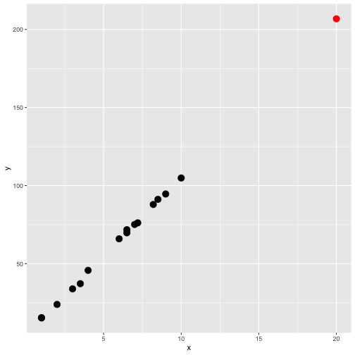<!-- --> ] .pull-right[ 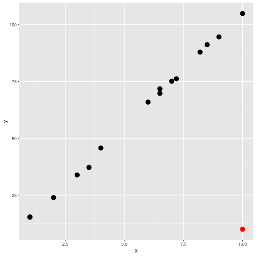<!-- --> ] --- ## Outliers should be carefully studied for 1. why they occurred and 2. whether they should be retained in the model. --- ##Types of outliers that occur in the context of regression 1. regression outlier 2. residual outlier 3. x-space outlier 4. y-space outlier 5. x- and y-space outlier --- ## 1. Regression outlier - lies off the line fit to the other 15 observations - determined from the remaining `\((n-1)\)` observations. 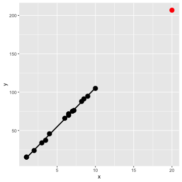<!-- --> --- ## 2. Residual outlier A point that has large standardized or studentized residual when it is used with all `\(n\)` observations to fit a model. .pull-left[ 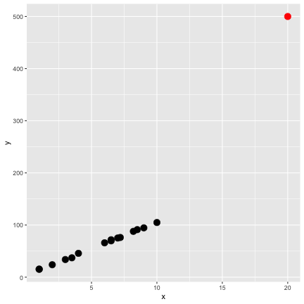<!-- --> ] .pull-right[ ``` y x 1 15.37697 1.0 2 15.30155 1.0 3 23.90198 2.0 4 33.86959 3.0 5 37.20347 3.5 6 45.72057 4.0 7 65.93912 6.0 8 69.77062 6.5 9 71.75913 6.5 10 75.11737 7.0 11 76.14688 7.2 12 87.90926 8.2 13 91.19637 8.5 14 94.62842 9.0 15 104.87674 10.0 16 500.00000 20.0 ``` ] --- ## 2. Residual outlier (cont.) ```r lmfit <- lm(y~x, data=example.data) library(broom) augment(lmfit) ``` ``` # A tibble: 16 × 8 y x .fitted .resid .hat .sigma .cooksd .std.resid <dbl> <dbl> <dbl> <dbl> <dbl> <dbl> <dbl> <dbl> 1 15.4 1 -35.7 51.0 0.157 46.3 0.130 1.18 2 15.3 1 -35.7 51.0 0.157 46.3 0.129 1.18 3 23.9 2 -13.0 36.9 0.125 47.5 0.0505 0.840 4 33.9 3 9.63 24.2 0.100 48.3 0.0165 0.543 5 37.2 3.5 21.0 16.2 0.0902 48.6 0.00651 0.362 6 45.7 4 32.3 13.4 0.0816 48.6 0.00396 0.298 7 65.9 6 77.6 -11.6 0.0632 48.7 0.00220 -0.256 8 69.8 6.5 88.9 -19.1 0.0625 48.5 0.00588 -0.420 9 71.8 6.5 88.9 -17.1 0.0625 48.5 0.00472 -0.376 10 75.1 7 100. -25.1 0.0634 48.3 0.0103 -0.552 11 76.1 7.2 105. -28.6 0.0642 48.1 0.0136 -0.629 12 87.9 8.2 127. -39.5 0.0720 47.4 0.0295 -0.872 13 91.2 8.5 134. -43.0 0.0756 47.2 0.0370 -0.951 14 94.6 9 146. -50.9 0.0828 46.5 0.0577 -1.13 15 105. 10 168. -63.3 0.102 45.1 0.115 -1.42 16 500 20 395. 105. 0.641 1.14 12.5 3.74 ``` --- ## 2. Residual outlier (cont.) Distribution of `.std.resid` in the previous output. 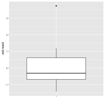<!-- --> --- ## 3. X-space outlier .pull-left[ 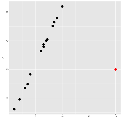<!-- --> ] .pull-right[ ### Hight leverage point A data point can be unusual in its x variables. ] --- ## 4. Y-space outlier .pull-left[ 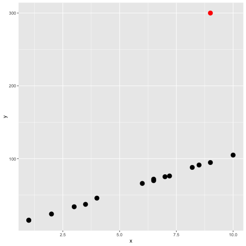<!-- --> ] .pull-right[ ### High discrepancy point A point has an unusual y-value given its x-value. ] --- ## 5. X- and Y-space outlier .pull-left[ <!-- --> ] .pull-right[ point that has both high leverage and high discrepancy ] --- ## Least-squares regression fit .pull-left[ 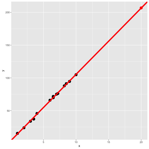<!-- --> ] .pull-right[ 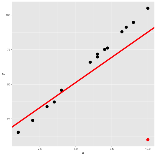<!-- --> ] Red line: all data including the red point. --- ## Least-squares regression fit .pull-left[ 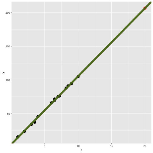<!-- --> ] .pull-right[ 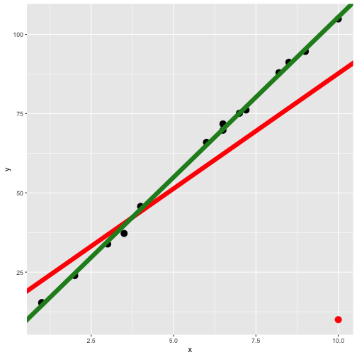<!-- --> ] Red line: all data including the red point. Green line: for all black point (without red point). --- ## Assessing leverage **Hat (leverages) value:** Helps to identify extreme `\(X\)` values. **In simple linear regression** `$$h_{ii} = \frac{1}{n} + \frac{(x_i-\bar{x})^2}{\sum_{j=1}^n(x_j - \bar{x})^2},$$` where `\(i = 1, 2, ... n\)` Hat value is bound between `\(1/n\)` and 1, with 1 denoting highest leverage. n - total number of points --- ## Assessing leverage (cont.) **In multiple linear regression** `\(Y = \beta_0 + \beta_1X_1 + \beta_2X_2 + ...+\beta_pX_p + \epsilon\)` .pull-left[ `$$Y = \begin{bmatrix} Y_{1}\\ Y_{2}\\ .\\ .\\ .\\ Y_{n} \end{bmatrix}$$` ] .pull-right[ `$$X = \begin{bmatrix} 1 \text{ } x_{11} \text{ } x_{12} \text{ } ... \text{ } x_{1p}\\ 1 \text{ } x_{21} \text{ } x_{22} \text{ } ... \text{ }x_{2p}\\ .\\ .\\ .\\ 1 \text{ } x_{n1} \text{ } x_{n2} \text{ }...\text{ } x_{np} \end{bmatrix}$$` ] `$$H = X(X'X)^{-1}X'$$` Hat matrix diagonal is a standardized measure of the distance of the `\(i\)`th observation from the center (or centroid) of the `\(x-\)`space. The leverage (hat) value `\(h_{ii}\)` does not depend on the response `\(Y_i\)`. --- ## Assessing leverage: Example .pull-left[ 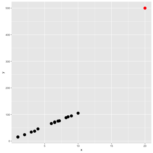<!-- --> ] .pull-right[ ``` y x 1 15.37697 1.0 2 15.30155 1.0 3 23.90198 2.0 4 33.86959 3.0 5 37.20347 3.5 6 45.72057 4.0 7 65.93912 6.0 8 69.77062 6.5 9 71.75913 6.5 10 75.11737 7.0 11 76.14688 7.2 12 87.90926 8.2 13 91.19637 8.5 14 94.62842 9.0 15 104.87674 10.0 16 500.00000 20.0 ``` ] --- ## Assessing leverage: Example (cont) ```r library(broom) data.fit <- lm(y ~x, data=example.data) augment(data.fit) ``` ``` # A tibble: 16 × 8 y x .fitted .resid .hat .sigma .cooksd .std.resid <dbl> <dbl> <dbl> <dbl> <dbl> <dbl> <dbl> <dbl> 1 15.4 1 -35.7 51.0 0.157 46.3 0.130 1.18 2 15.3 1 -35.7 51.0 0.157 46.3 0.129 1.18 3 23.9 2 -13.0 36.9 0.125 47.5 0.0505 0.840 4 33.9 3 9.63 24.2 0.100 48.3 0.0165 0.543 5 37.2 3.5 21.0 16.2 0.0902 48.6 0.00651 0.362 6 45.7 4 32.3 13.4 0.0816 48.6 0.00396 0.298 7 65.9 6 77.6 -11.6 0.0632 48.7 0.00220 -0.256 8 69.8 6.5 88.9 -19.1 0.0625 48.5 0.00588 -0.420 9 71.8 6.5 88.9 -17.1 0.0625 48.5 0.00472 -0.376 10 75.1 7 100. -25.1 0.0634 48.3 0.0103 -0.552 11 76.1 7.2 105. -28.6 0.0642 48.1 0.0136 -0.629 12 87.9 8.2 127. -39.5 0.0720 47.4 0.0295 -0.872 13 91.2 8.5 134. -43.0 0.0756 47.2 0.0370 -0.951 14 94.6 9 146. -50.9 0.0828 46.5 0.0577 -1.13 15 105. 10 168. -63.3 0.102 45.1 0.115 -1.42 16 500 20 395. 105. 0.641 1.14 12.5 3.74 ``` --- ## Assessing leverage: Example (cont) `$$\text{cut off} = \frac{2p}{n},$$` `\(p\)` - number of predictors/ x- variables. `\(n\)` - number of observations. In this case `$$\text{cut off} = \frac{2p}{n} = \frac{2 \times 1}{16} = 0.125$$` We say a point is a high leverage point if `$$h_{ii} > \frac{2p}{n}$$` This cut off does not apply `\(\frac{2p}{n} > 1\)`. --- ## What to do when you find outliers? - Explore! (data entry errors, recording errors, etc.) --- ## Influence - a point with high leverage can dramatically impact the regression model. .pull-left[ **All points (red)** <!-- --> ] .pull-right[ **Only black points (green)** <!-- --> ] - Influence - measures how much impact a point has on the regression model --- ## Measure of Influence (cont.) [Cook's distance](https://en.wikipedia.org/wiki/Cook%27s_distance), `\(D_i\)`, is a measure of influence. ```r augment(data.fit) ``` ``` # A tibble: 16 × 8 y x .fitted .resid .hat .sigma .cooksd .std.resid <dbl> <dbl> <dbl> <dbl> <dbl> <dbl> <dbl> <dbl> 1 15.4 1 -35.7 51.0 0.157 46.3 0.130 1.18 2 15.3 1 -35.7 51.0 0.157 46.3 0.129 1.18 3 23.9 2 -13.0 36.9 0.125 47.5 0.0505 0.840 4 33.9 3 9.63 24.2 0.100 48.3 0.0165 0.543 5 37.2 3.5 21.0 16.2 0.0902 48.6 0.00651 0.362 6 45.7 4 32.3 13.4 0.0816 48.6 0.00396 0.298 7 65.9 6 77.6 -11.6 0.0632 48.7 0.00220 -0.256 8 69.8 6.5 88.9 -19.1 0.0625 48.5 0.00588 -0.420 9 71.8 6.5 88.9 -17.1 0.0625 48.5 0.00472 -0.376 10 75.1 7 100. -25.1 0.0634 48.3 0.0103 -0.552 11 76.1 7.2 105. -28.6 0.0642 48.1 0.0136 -0.629 12 87.9 8.2 127. -39.5 0.0720 47.4 0.0295 -0.872 13 91.2 8.5 134. -43.0 0.0756 47.2 0.0370 -0.951 14 94.6 9 146. -50.9 0.0828 46.5 0.0577 -1.13 15 105. 10 168. -63.3 0.102 45.1 0.115 -1.42 16 500 20 395. 105. 0.641 1.14 12.5 3.74 ``` --- ## Measure of Influence (cont.) - We usually consider points for which `\(D_i > 1\)` to be influential (Montgomery, et al.). ``` # A tibble: 16 × 8 y x .fitted .resid .hat .sigma .cooksd .std.resid <dbl> <dbl> <dbl> <dbl> <dbl> <dbl> <dbl> <dbl> 1 15.4 1 -35.7 51.0 0.157 46.3 0.130 1.18 2 15.3 1 -35.7 51.0 0.157 46.3 0.129 1.18 3 23.9 2 -13.0 36.9 0.125 47.5 0.0505 0.840 4 33.9 3 9.63 24.2 0.100 48.3 0.0165 0.543 5 37.2 3.5 21.0 16.2 0.0902 48.6 0.00651 0.362 6 45.7 4 32.3 13.4 0.0816 48.6 0.00396 0.298 7 65.9 6 77.6 -11.6 0.0632 48.7 0.00220 -0.256 8 69.8 6.5 88.9 -19.1 0.0625 48.5 0.00588 -0.420 9 71.8 6.5 88.9 -17.1 0.0625 48.5 0.00472 -0.376 10 75.1 7 100. -25.1 0.0634 48.3 0.0103 -0.552 11 76.1 7.2 105. -28.6 0.0642 48.1 0.0136 -0.629 12 87.9 8.2 127. -39.5 0.0720 47.4 0.0295 -0.872 13 91.2 8.5 134. -43.0 0.0756 47.2 0.0370 -0.951 14 94.6 9 146. -50.9 0.0828 46.5 0.0577 -1.13 15 105. 10 168. -63.3 0.102 45.1 0.115 -1.42 16 500 20 395. 105. 0.641 1.14 12.5 3.74 ``` <!--Interpretations: page 213--> --- ## Leverage and Influence Remember that leverage alone does not mean a point exerts high influence, but it certainly means it's worth investigating. --- ## Influence - An **influence point**, can make a noticeable impact on the model coefficients in that it pulls the regression model in its direction. .pull-left[ **All points** 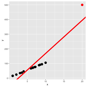<!-- --> ] .pull-right[ **Only black points (green)** 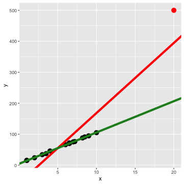<!-- --> ] --- ## Other Measures of Influence - DEFITS and DFBEATAS ## Treatment of Influential Observations - Should influential points ever be discarded? If there is a recording error, measurement error, or if the sample point is invalid or not part of the population that was intended to be sampled, then deleting the point is appropriate. - The field of **robust statistics** is concerned with more advanced methods of dealing with influential outliers. For e.g.: **down weight** observations in proportional to residual magnitude or influence. Then highly influential observations will receive less weight than they would in a least-squares fit. e.g: Robust regression <!--The field of robust statistics is concerned with more sophisticated ways of dealing with outliers--> --- class: center, middle Acknowledgement Introduction to Linear Regression Analysis, Douglas C. Montgomery, Elizabeth A. Peck, G. Geoffrey Vining All rights reserved by [Dr. Thiyanga S. Talagala](https://thiyanga.netlify.app/)